Mountain car, Q-learning, and Experience Replay with Pytorch

Hey there!

Mountain Car (MC) is a classic Reinforcement Learning (RL) problem. It was briefly shown in a video I was watching, so I figured I’d give it a shot.

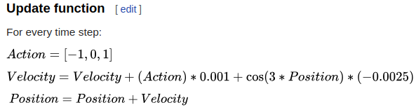
The first thing I did was whip up a little display that could show a given episode, which turns out to be invaluable for debugging, etc. I started by defining the landscape as a function y = f(x), where x is the horizontal position of the car. The display shows a handful of things:

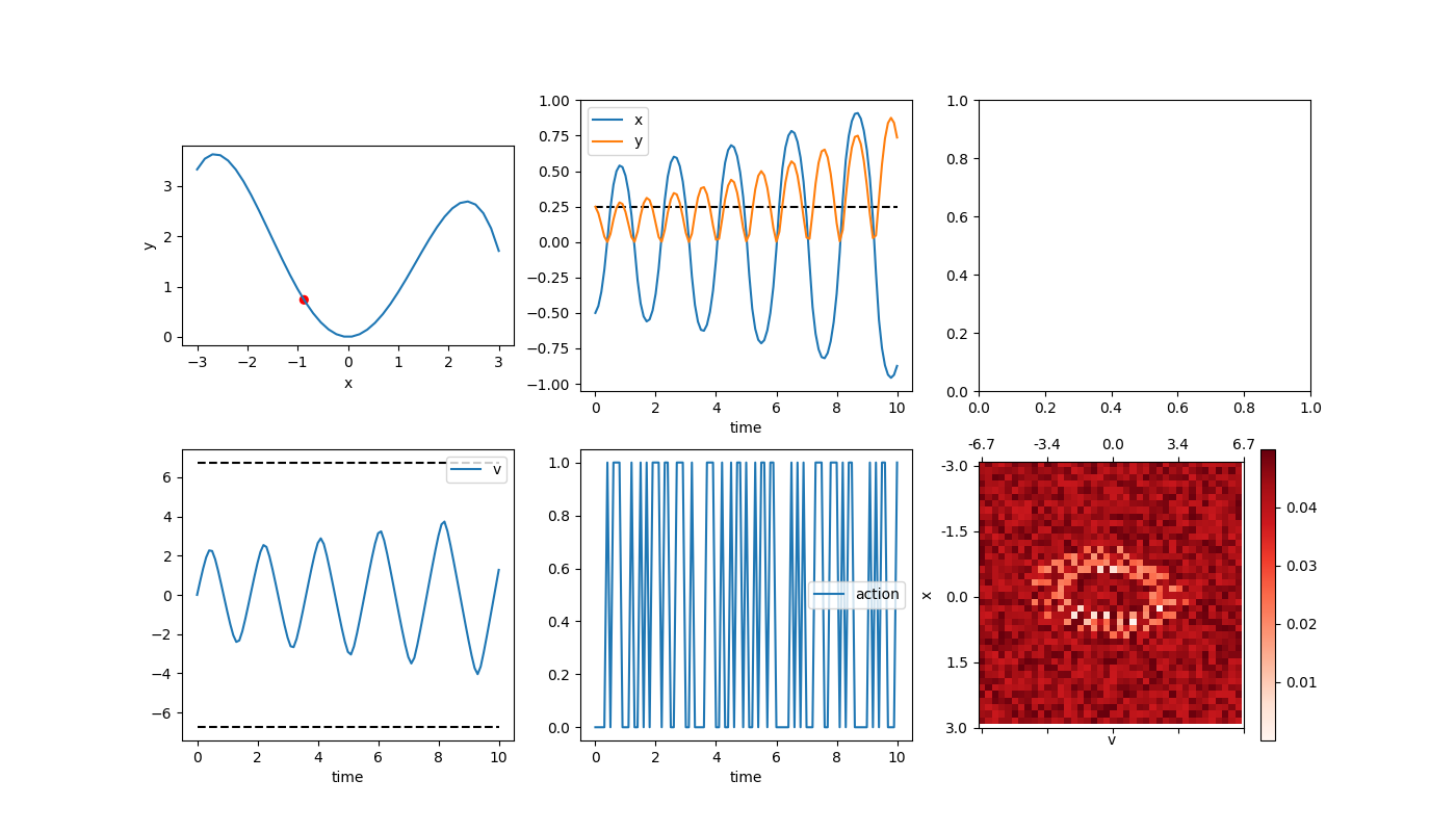
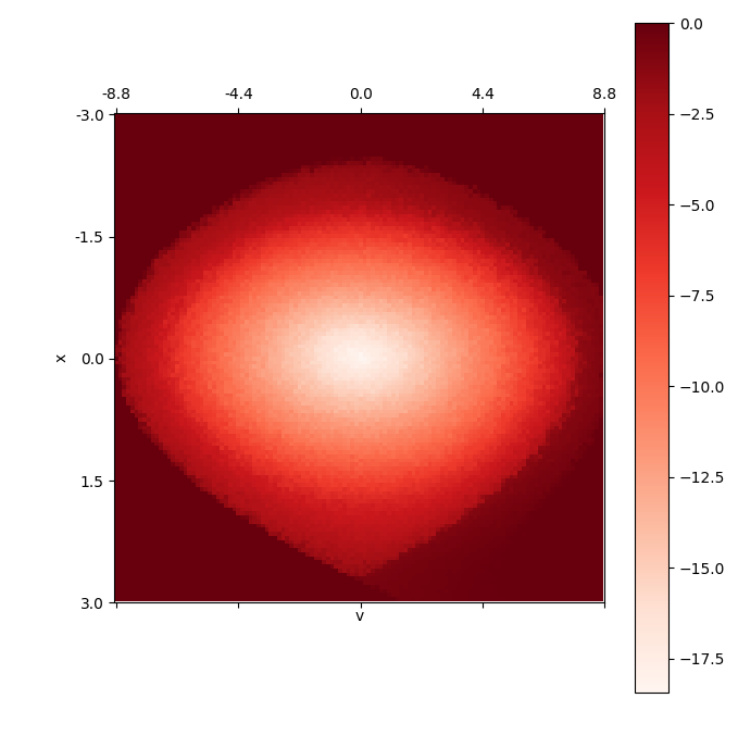
The upper left is the landscape, and the red dot is the current position of the car. The top middle are a plot of the x and y positions. The bottom left is the velocity. The bottom middle is the current action taken (forward or backward, I didn’t give it a “do nothing” option). The bottom right is the value function approximation, which I’ll talk about more later. I’ll sometimes put stuff in the top right, but generally don’t have anything in it.

The first little confusion was getting the mechanics right. At a given point on the landscape, the car is under the force of gravity and the applied force from its wheels. Gravity is always down, but produces a force tangential to the slope wherever the car is. The applied force is also in that direction. So this is pretty easy to iterate through using something like the Euler-Cromer method (which is supposedly a little more robust to gaining energy over time than the regular Euler method). However, when I ran it with a timestep of dt = 0.1, and no applied forces, having it start at x0 = -0.5 (so it has some potential energy to begin with), it gives:

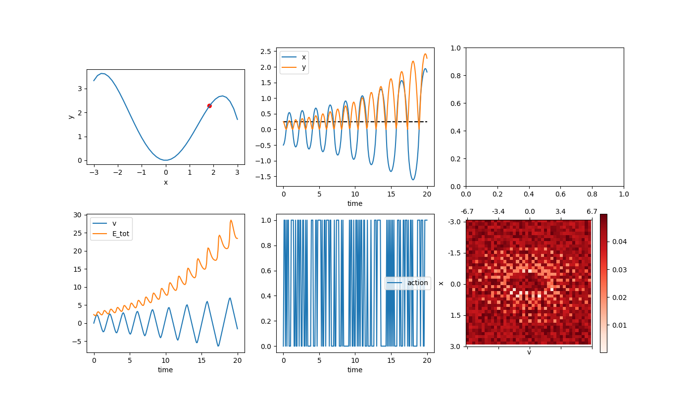
You can see that it’s going higher and higher. I also plotted the total energy in the bottom left (which won’t be super useful when we let the car apply a force in the future because then it won’t be conserved, but is now), which you can also see increasing. Now, the Euler method is “physically correct” in the sense that it’s literally just the equations of motion for a particle, but because of the finite time step it diverges from reality (which uses an “infinitesimal time step”). So, you can get better accuracy over the same time if you use a smaller dt and more steps, like so (dt = 0.01):

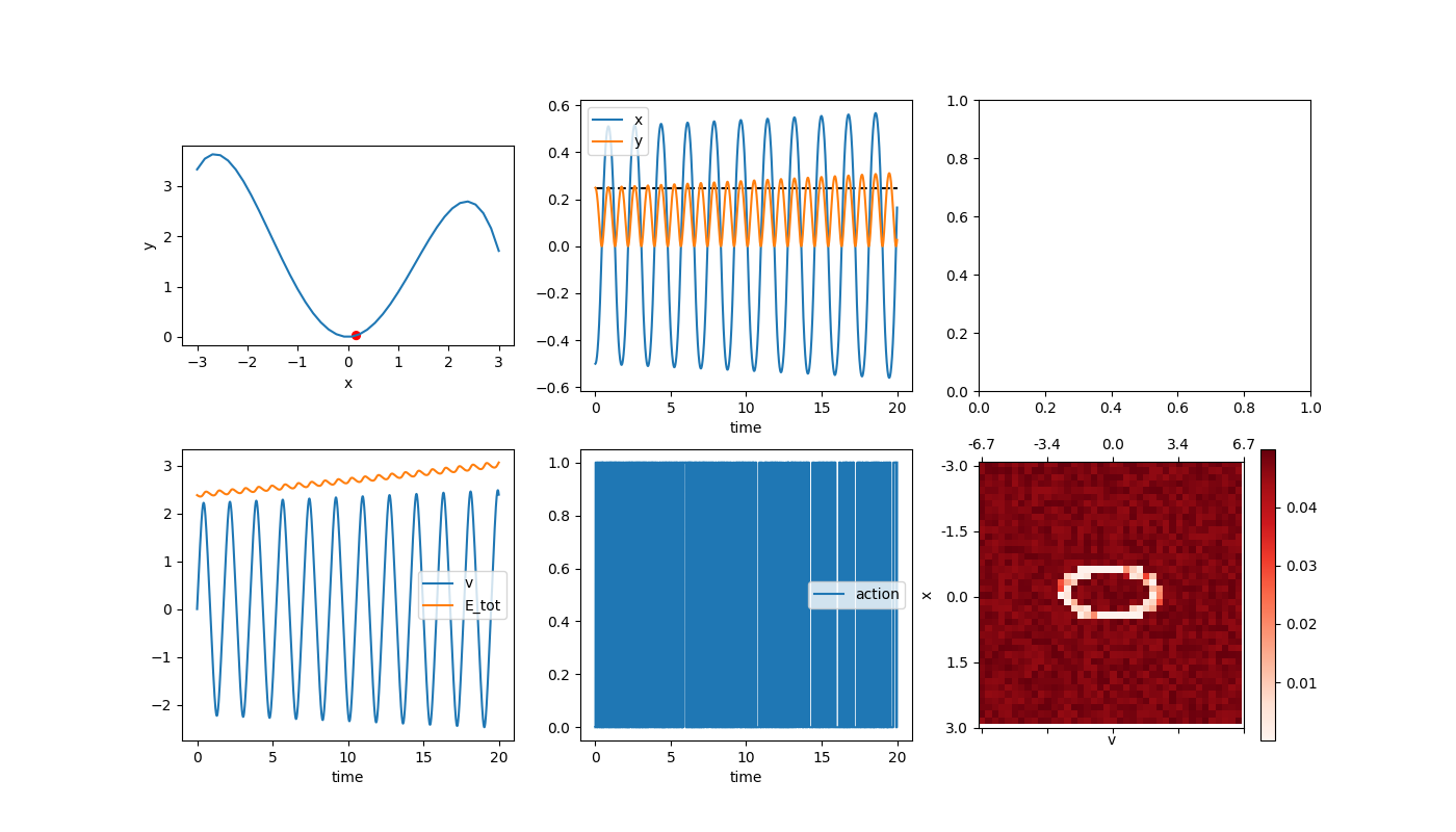
It’s definitely growing more slowly, but still also bad (and it will make us have to compute more anyway). I think we especially don’t want the energy growing unnaturally in a problem where the goal is to learn to do something similar. So, another alternative is using a better integrating strategy, like 4th order Runge Kutta (RK4). Using the original time step (dt = 0.1), this gives:

About as good as the E-C method with dt = 0.01, but more importantly, it’s losing energy rather than gaining it, which is better. This just adds a bit of a hurdle for us, but at least can’t be cheating.

As a brief aside, I went through a bunch of trouble, making sure the mechanics were accurate and stuff, but if you look at the Wikipedia article, this is what they use to update the velocity:

I kind of suspected that what I was doing (calculating the slope at each RK4 point, etc) might be overkill because the differences in the acceleration due to gravity at different points in the same time step are probably negligible, but I guess you can really be pretty loose with it and the mechanics will still probably work out? Oh well.

Anyway, now time to implement the RL part! There are a handful of ways to set the problem up, but maybe the most common is discretizing the parameter space to form the feature vector, as also briefly mentioned in the wiki article. The idea is that if you know your x coordinate ranges from [-1,1] and your velocity will always be in the range [-5,5], that marks out a section of the 2D x-v plane. You can then chop this plane up into smaller squares, such that for any (x,v) combo within that section, it will be in one of those discretized squares, which will be the car’s current state. I chose to discretize it in 40 subsections for each dimension, so there are 1600 states.

So, the state S is a function of x and v, S(x,v). So, the value function V(S) is a 40×40 array, and the state-action value function Q(S,A) is a 40x40x2 matrix, because there are only 2 actions to take. In reality, I’m actually implementing it so V and Q are each the matrix dot product of a feature vector X(S,A) and a weights vector : , and technically is the thing we’ll be trying to improve. But, this will probably be mostly hidden this time, so don’t worry about it.

I implemented TD(0), TD() (TDL), and Experience Replay using batch gradient descent. I’ll go over TD(0) first.

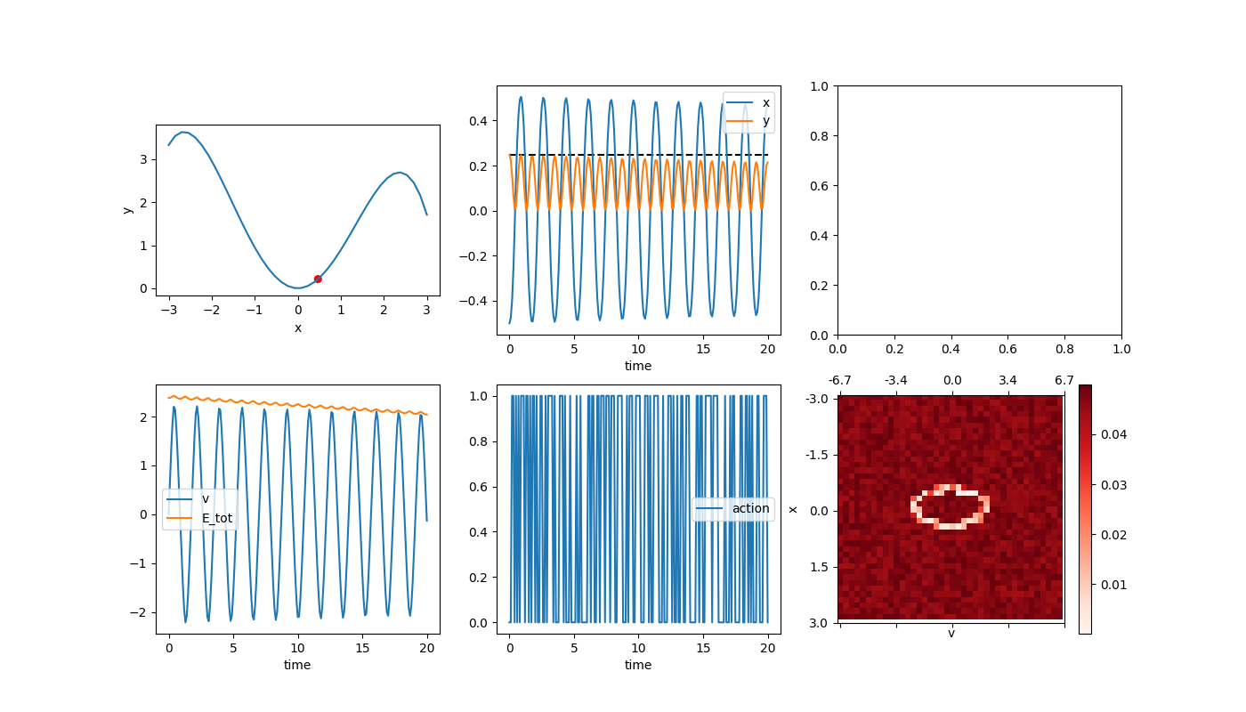
For TD(0), here’s an example of an episode. I set the acceleration of the car to be some fraction of the gravitational acceleration, in each problem. Here the fraction is 0.1, which I’ll mostly use. As a point of reference, if you can accelerate with , that would mean that you can only go up a ~5 degree slope, so it’s not super easy for the car on this slope. There will technically always be an e-greedy policy, but for now I’m setting so it is greedy. I’ll have dt = 0.1 for this whole post, and for now . Here, , but I’ll talk about that in the future. Here’s what it looks like when it finishes the episode:

You can see that 1) it takes ~4,000 steps (400/0.1) to complete, 2) it gets pretty far often, and then gets worse, before getting better, 3) the value function is definitely getting a lot of character.

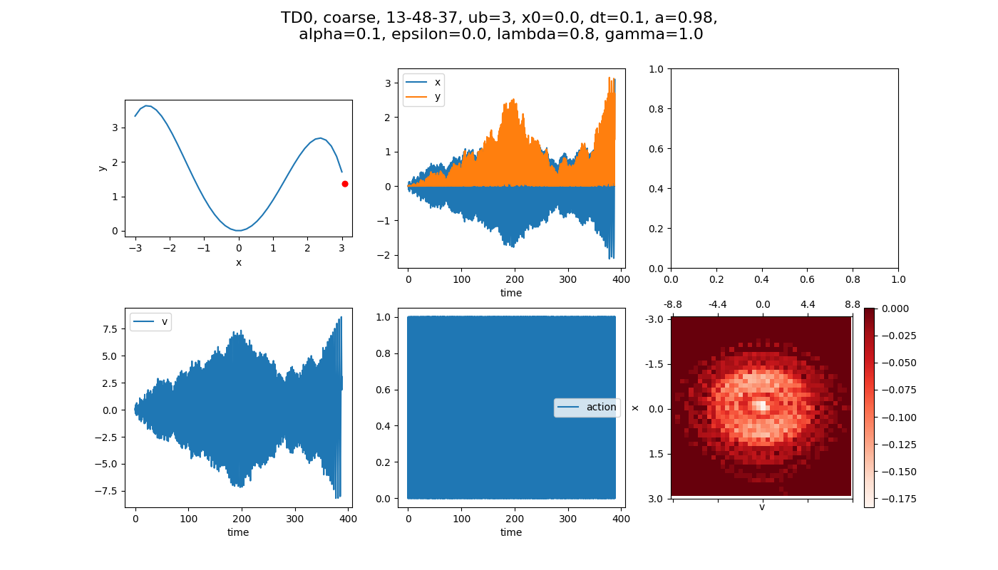
We can then run the same thing, but over many episodes, keeping the value of Q(S,A) we’ve found so far, so that it will use it and continue to improve it. This is a standard way of showing that the system is learning over time, because the steps it takes for an episode to complete should decrease.

And, lo and behold, it does:

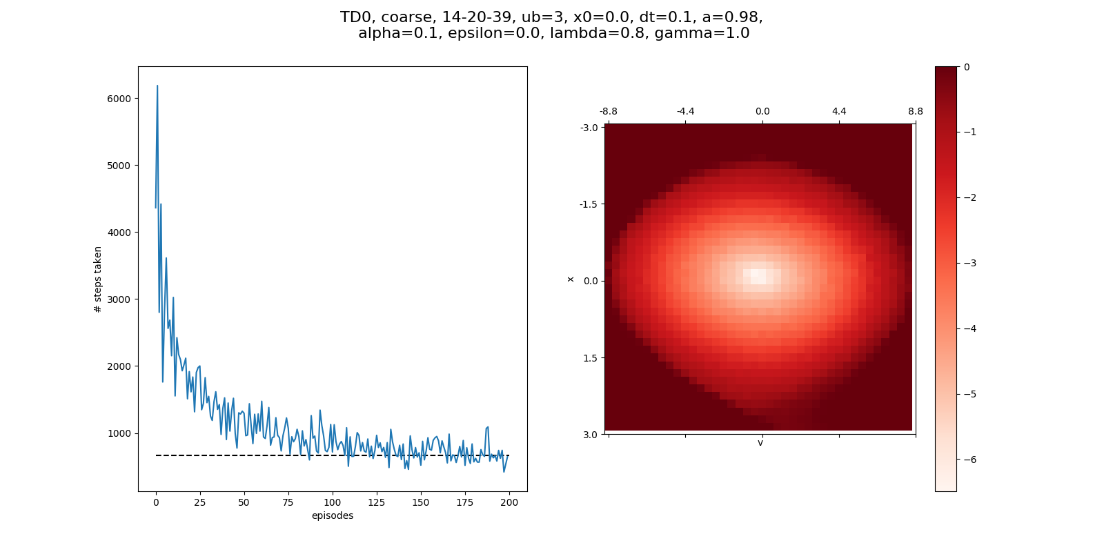
After 200 episodes, it needs about 800 steps to complete. You can see that if we run it longer, with 3000 episodes, it converges a little more, now more like 300 steps:

Now let’s try working some greediness into this. It’s doing fine with total greediness, but maybe if we introduce some randomness early on, it might find better states, or converge faster? For clarity, I’m not resetting between episodes, which I think makes more sense.

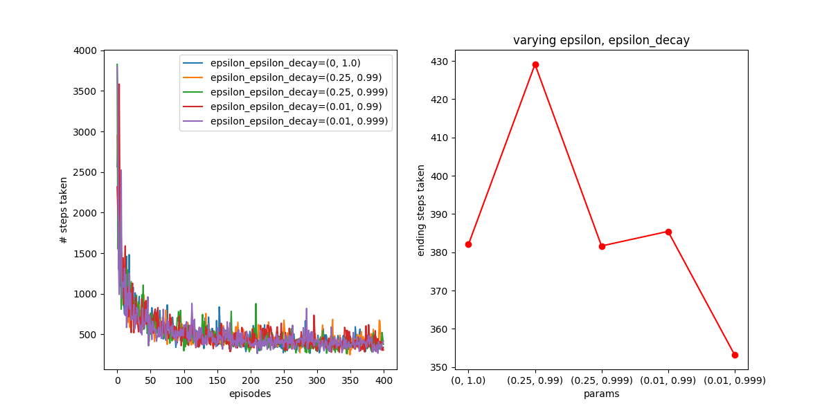
Hmm. It turns out epsilon greediness doesn’t seem to have a huge effect, at least for the values I tried. For clarity, epsilon_decay is the value that is multiplied by epsilon every time step to get the new value. On the right I’m plotting the average of the last 20 points of each curve on the left, to show where they settle. So it seems like it just doesn’t do much here.

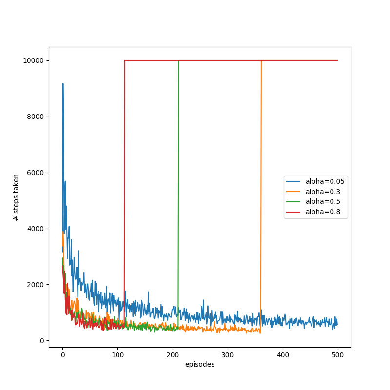
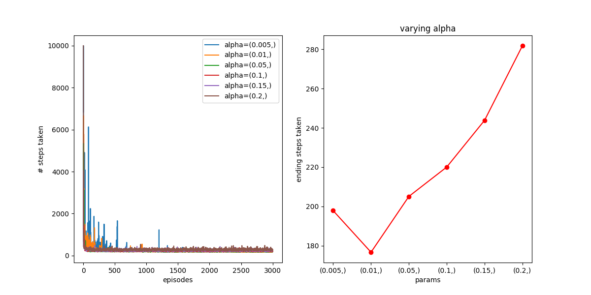
A parameter that has lots of effect is the learning rate, alpha. Here it is for a shorter time scale:

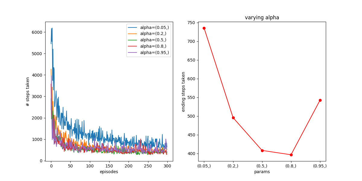
You can see that the higher values converge faster, though it seems like may be too high and cause noise. Here it is over a longer time scale:

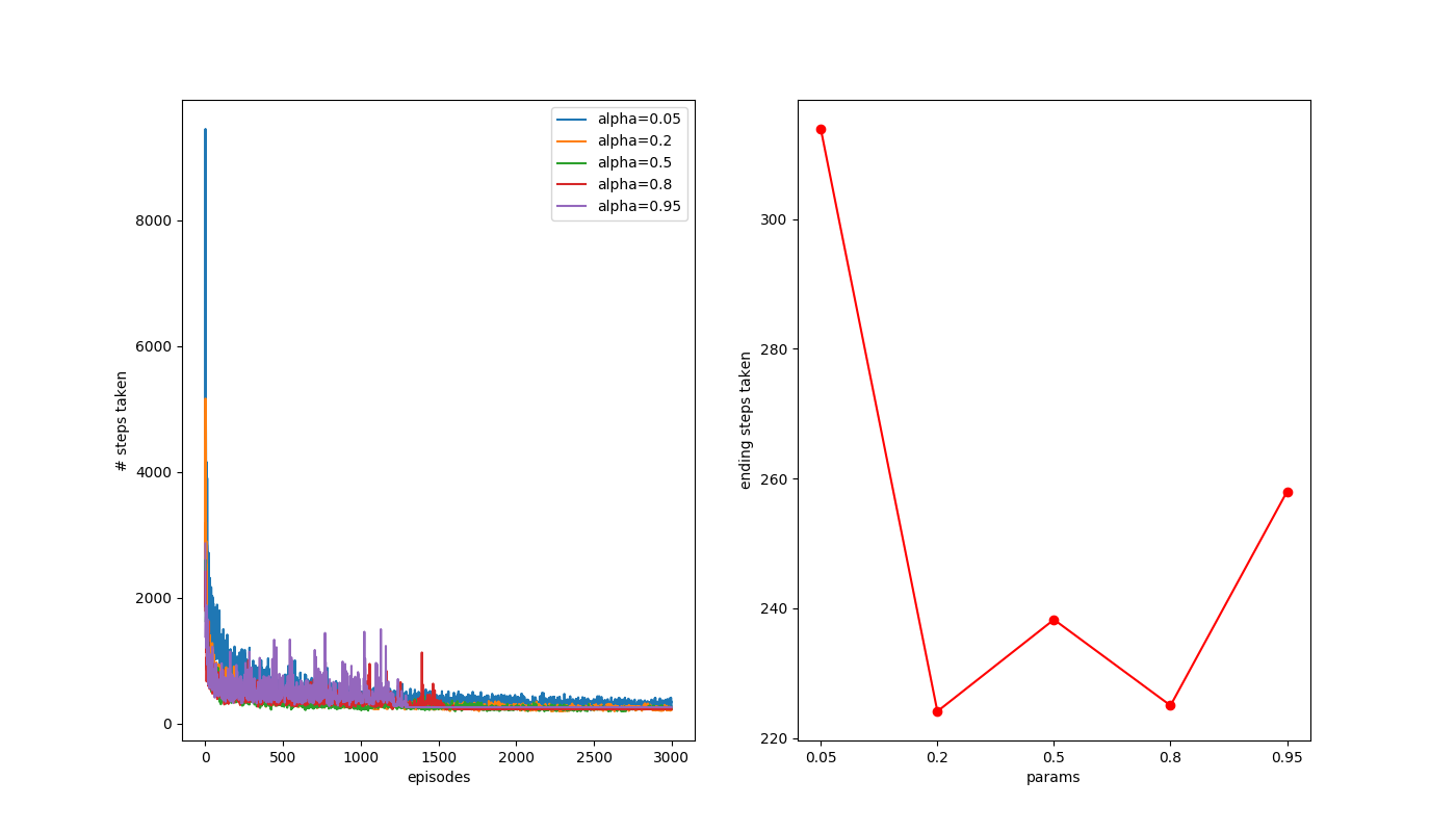
Similar story for this one too, though by this point the differences between = [.2, .5, .8] are probably just due to noise.

A couple more weird things. First, using TD(), and varying with , greedy actions, and 400 episodes also shows not much dependence:

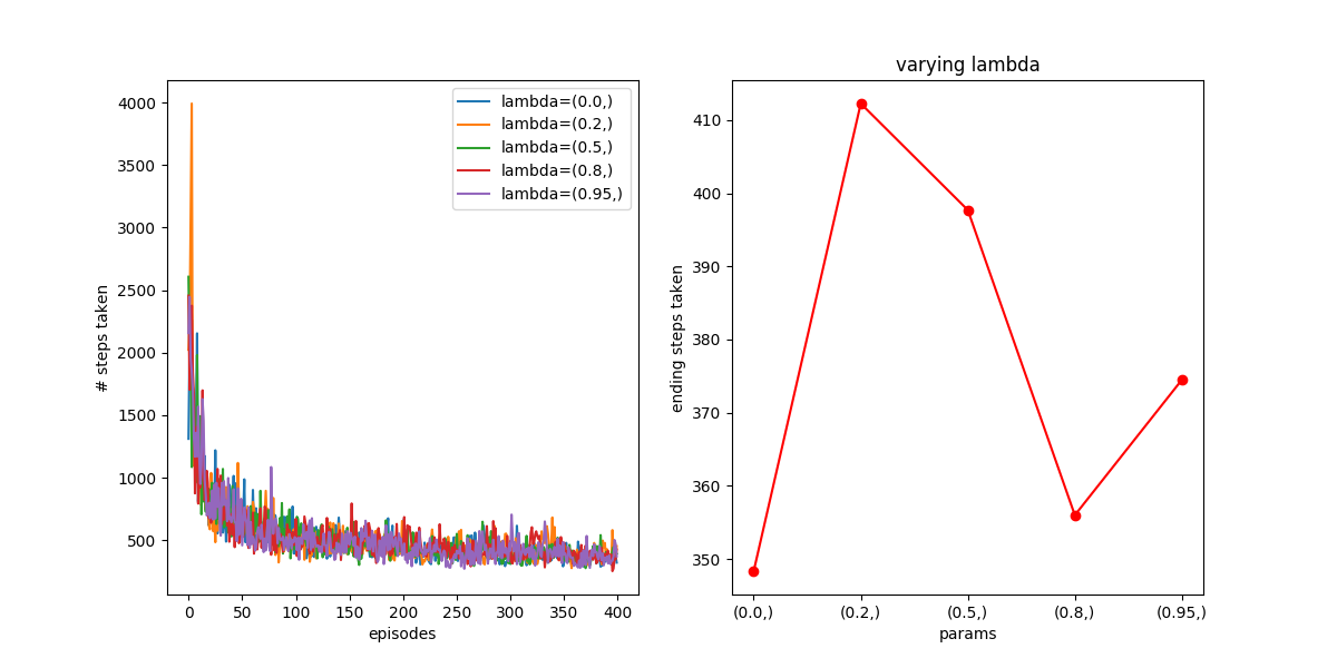
Weird! How about for 3,000 episodes?

Next, let’s look at . This one’s a puzzler. I was originally using as a default for testing other stuff, and found that it was causing higher values to show improvement over episodes, but at some point just “snap” and always take the maximum number of steps per episode I was allowing. This is pretty confusing, because I know that if you use bad values, things can not converge, etc, but I always assumed that would happen pretty quickly, as opposed to showing good results, and then occurring. For example, here I vary with :

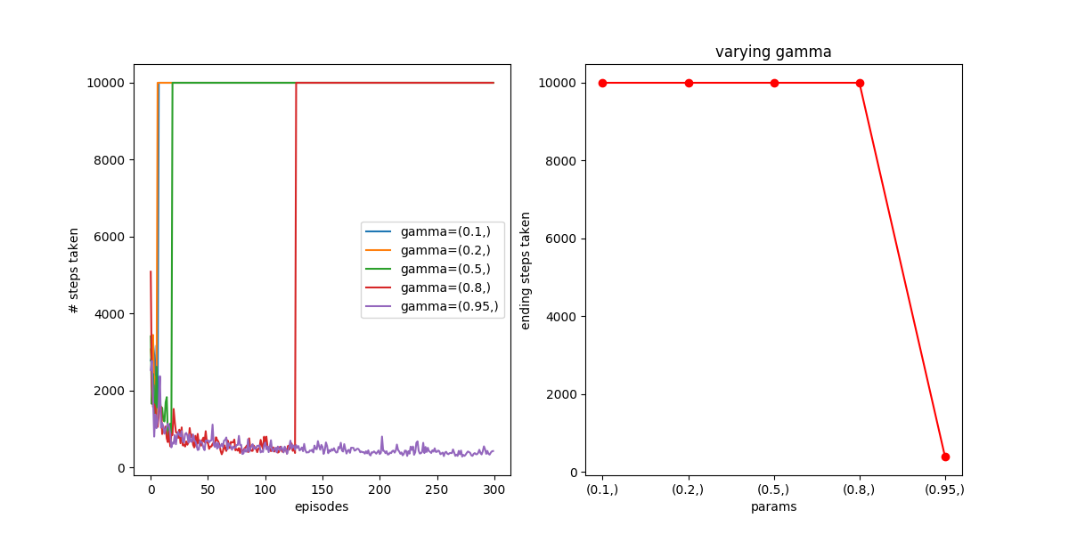
works okay, but the rest “break” early on, earlier for lower numbers of . Like I mentioned above, here’s keeping a “bad” value of and varying instead:

So for this, works if it’s low enough, but the combo of “low” (0.8) and a higher breaks it. Hmmm.

Let’s look at a few other things. First, something I was curious about is the effect of the discretization size (i.e., how finely x and v are chopped up) in the coarse coding. By default, I was using 40 for each of x and v, but it’s not clear to me how that number would change things. On the one hand, it seems like finer is probably better, because a single entry of the Q matrix will represent a more specific range of (x,v), and therefore be able to more finely tune its behavior to that range. On the other hand, the more finely you dice the parameter space, the less samples each block has, so it will be much slower to learn. For example, the agent  probably should do the exact same thing for the two states (x=-1, v=1) and (x=-1.5,v=1) (i.e., accelerate towards positive x), but if these states are considered different, it’ll have to learn stuff for them separately, which is way less efficient.

Anyway, here’s what I found, varying from 10 to 80 discretizations. Here, is 0.7, the default I’m using for most runs now (since I determined it’s the best if ):

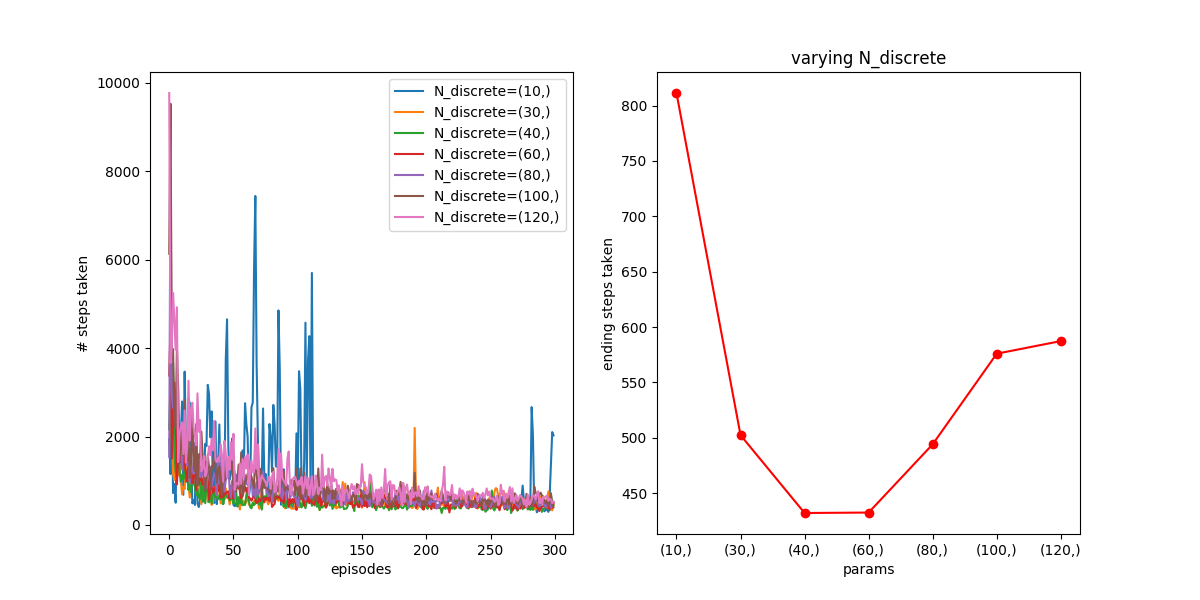
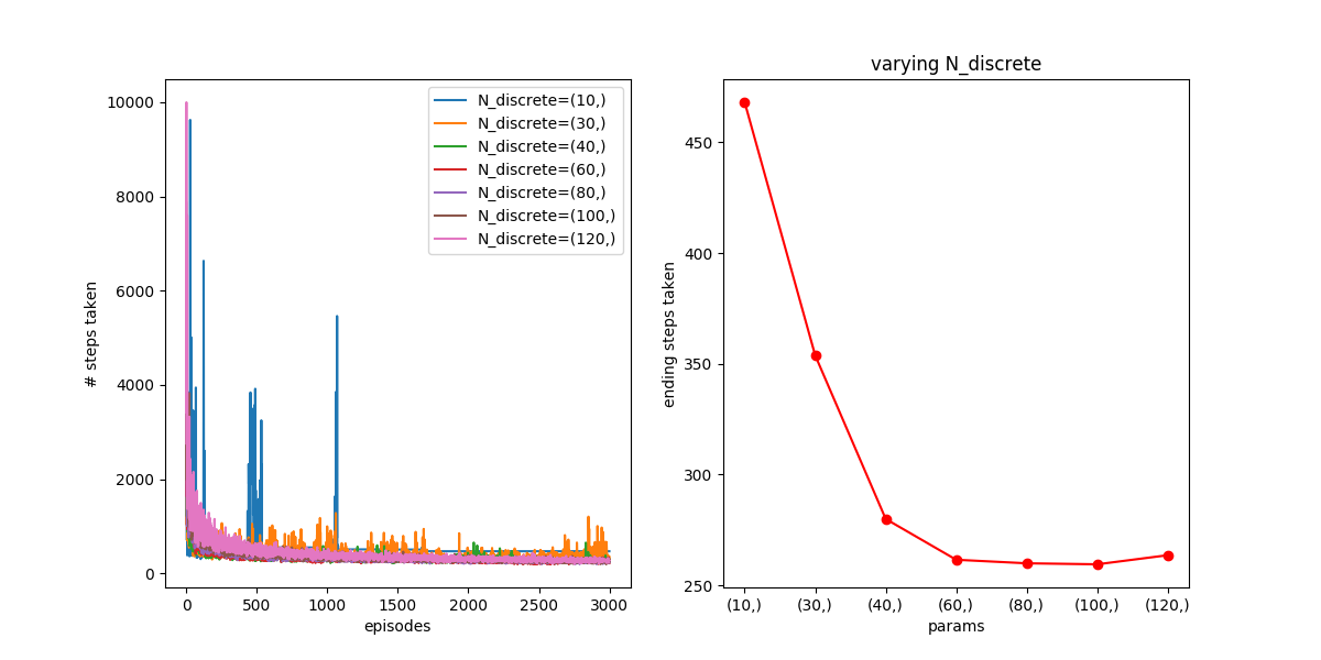
You can see that for both 300 and 3000, N=10 is just too small to describe the different “states” the car is in, so it never does great. For the higher N’s, like N=100 and N=120, you can see that they don’t get enough samples for the 300 one, so don’t converge great, but with the 3000 one, they get enough samples and are about as good as N=60.

Out of curiosity, I plotted only N=10 and N=60 together, but with the original , but also a smaller . When you do that, this effect is really pronounced!

:

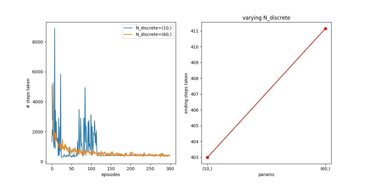
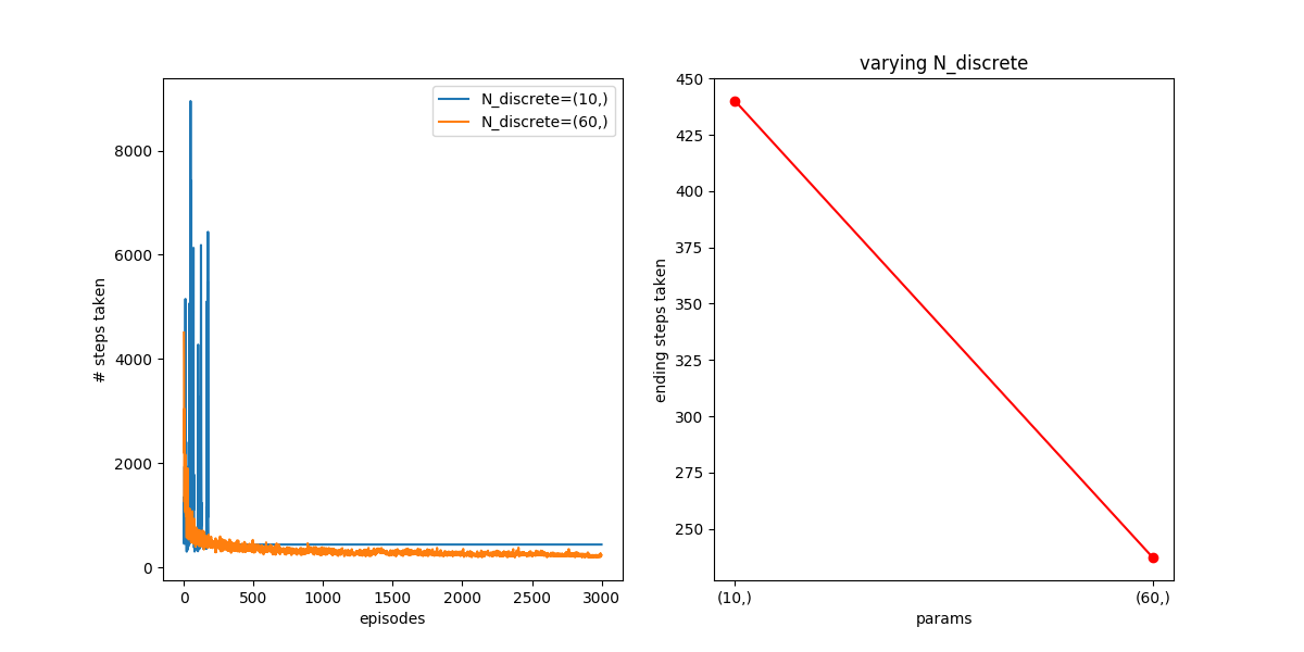
For 300 episodes, they’re pretty much the same. However, after 3000, the N=60 one has continued to improve, because it got more info it needed and was able to use it, while the N=10 one is about the same.

:

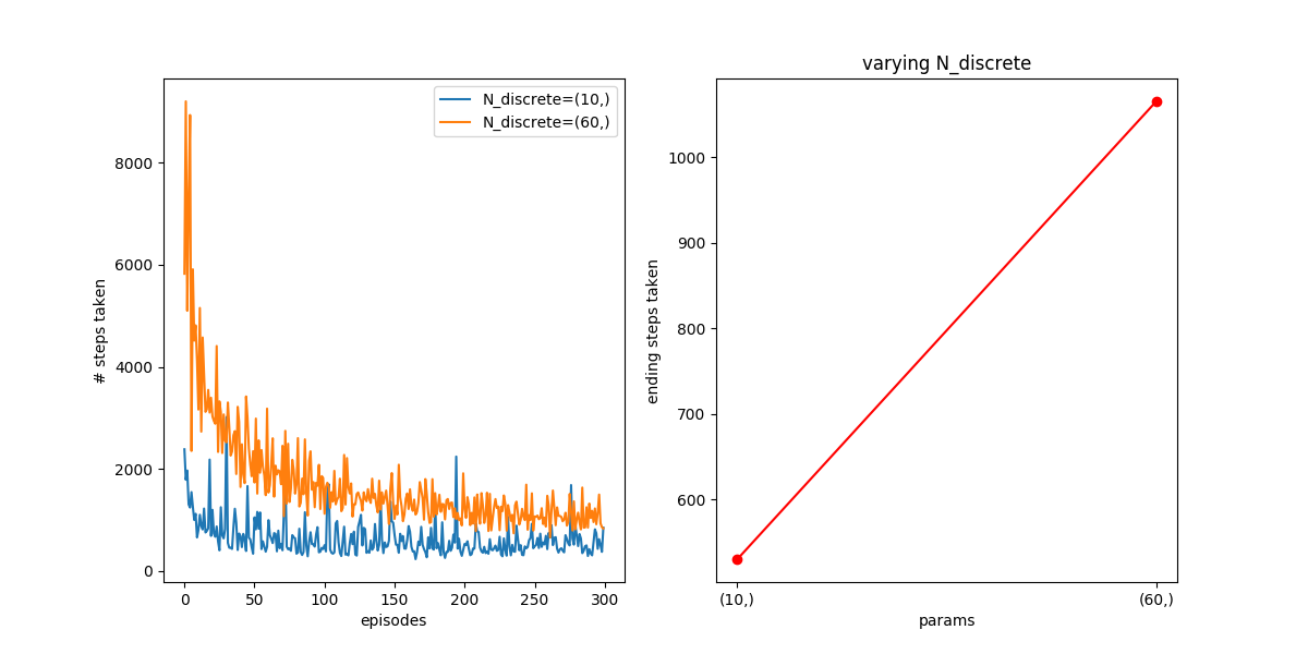
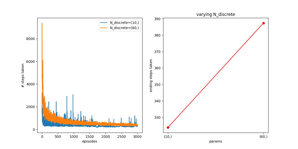
Here, you can see that if you try a smaller learning rate, the effect is really pronounced. After 300 episodes, N=10 has converged quickly, but N=60 is both getting fewer samples per state, and additionally, the smaller alphas mean that each samples “counts” for less. So, even after 3000, N=10 is somewhat better, though it seems like N=60 is still improving.

As an aside, the value function for N=120 looks great:

The last thing I’ll talk about today is using Experience Replay (ER), which is a technique used by Deepmind in solving the Atari games. The main gist is that, while the SARSA/TD/Q-learning stuff above basically continually updates Q based on steps it experiences at the moment, ER stores previous steps, and re-samples them again and again in a way that makes it more like a supervised learning problem.

In ER, you still choose actions the same way we have before, with -greedy, but each step, also store the “experience” (S,A,R,S’) of that step. That is, for a given S,A, performing action A will give you an R and the next state S’, so you store that whole outcome. In ER, you’ll also actually have two sets of weights, the “old”/”frozen” ones, and the “new” ones, that you’ll update. Periodically (every 20 time steps, say), you’ll copy the new weights to overwite the old ones.

Now, to update Q (or rather, its weights), every time step, you take a mini batch (maybe 20) of a random subset of those experiences. You then define the error/loss as the sum over , for all the experiences. Here, importantly, that term means, taking the maximum Q value you could get by choosing the best action A’ in state S’, using the “old” (or, “frozen”) weight values (that’s what the “w-” means). So you use a given experience (S,A,R,S’), but you don’t use whatever A’ you actually chose when that experience happened, you use the best one you could do now, using the current “frozen” weight values. Additionally, in the Q(S,A,w) term, (S,A) are given by the experience, but the actual value Q(S,A,w) is the one based on the current weights (hence the “w”).

The main motivation with ER is that you get to reuse data. Typically, in SARSA, you get to learn from an experience once. With ER, because you’re storing them, and a big part of the experience was the reward you got, it can converge faster because it’s using more info at each step.

To do this, I’m using pytorch. My weights matrix for Q is now also initialized as a tensor, which very conveniently shares the same memory as the numpy matrix it was originally. I’m using a batch size of 20 (fairly arbitrarily chosen) and an update period of 10 time steps (likewise) for copying the current weights to the “frozen” weights.

That said, here’s the function that cleanly replaces the previous updateTD0() or updateTDL() functions I was using before (in addition to a couple init things):

def batchUpdate(self):
    self.w_V = np.max(self.w_Q,axis=2)

    if self.iteration%self.frozen_update_period==0:
        self.updateFrozenQ()

    r = self.reward()

    (x_next,v_next) = (self.x_hist[-1],self.v_hist[-1])
    self.action_next = self.getAction(x_next,v_next)
    self.action_hist.append(self.action_next)

    S_ind = self.featureIndicesFromState(self.x,self.v)
    S_next_ind = self.featureIndicesFromState(x_next,v_next)

    experience = (S_ind,self.action,r,S_next_ind)

    self.samples_V.append(experience)
    self.samples_Q.append(experience)

    if len(self.samples_Q)>=self.N_batch:

        #Get random batch
        batch_Q_samples = sample(self.samples_Q,self.N_batch)

        #So this will be all the Q(s,a,w)'s  for the NEWEST w weights.
        X = torch.Tensor(np.zeros((self.N_batch,self.N_discrete,self.N_discrete,self.N_actions)))
        for i,samp in enumerate(batch_Q_samples):
            X[i,samp[0][0],samp[0][1],samp[1]] = 1

        #Calculate based on the CURRENT Q weights.
        Q_new = torch.sum(X.mul(self.w_Q_tensor),dim=[1,2,3])
        #Calculate based on the FROZEN Q weights.
        Q_old = torch.Tensor([max(self.w_Q_frozen[samp[3]]) for samp in batch_Q_samples])

        r = torch.Tensor([samp[2] for samp in batch_Q_samples])

        L = (r + self.gamma*Q_old - Q_new).pow(2).sum()
        L.backward()

        with torch.no_grad():
            self.w_Q_tensor -= self.alpha*self.w_Q_tensor.grad
            self.w_Q_tensor.grad.zero_()

It’s pretty much what I described above. So how does it do?

The first thing is to get an idea of what kind of value I need. To do this, I did the same as I did above, letting it learn for different values of :

Other plots I did for slightly lower (0.001) and higher (0.22) values make it very quickly blow up, so it seems like it’s fairly sensitive to , and needs a small one. It looks like is best for this. How does it compare to TD0, for its best value?

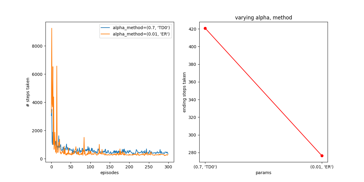
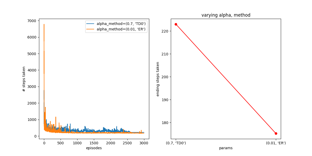
Hot damn! Not bad! You can see that it behaves better than TD(0) in both the short and long term, getting down to 175 steps in the end.

I scanned the batch size and frozen weights update period, too, but it didn’t seem super interesting so I’ll leave that out since this is already long.

Well, that’s all for now! There are a few things I’ll want to try in the future, so maybe I’ll come back to this.